Variable selection
In both statistical and theoretical models, we tend to work with a larger number of variables as once. A question, that will every researcher have to face very early on, is which variables to use in their models and which to leave out.
The answer to this question is far from easy. The appropriate way to determine which variables include depends on the goal of the analysis. In this section, we briefly mention techniques for predictive modeling and dedicate the rest of this chapter to variable selection for explanative models.
Predictive model
The main goal of predictive models is to achieve the best out-of-sample prediction. Consequently, variables in these models should be selected to maximize predictions for observations that were not used to compute the model.
The basic approach, best used for big data sets, is to split your data into three parts: training set, calibration set and testing set. The training set are the data used to estimate models. You can try estimating models with varying number of variables on them. Then you can compare their predictive performance on the calibration. Since the data in the calibration set haven’t been used for model estimation, it will give you an idea how will your model perform in the future. Once you picked one of the models, you can check its performance on the testing set, to get the final estimate of its usefulness.
More advanced approaches, often employed when data is too small to divide into three separate sets, are also available. The most common technique is called cross-validation. In this approach, the data are divided into k parts (called “folds”). Each model is then on the data from all folds except for one and the last of the folds is used as the calibration set to asses performance. This is done repeatedly with of the folds serving as the “calibration set” in turn and the performance is then averaged. For example, a 3 fold cross-validation would mean randomly splitting the data into three parts (folds). A model is then estimated on the data from fold 1 and 2, then checked on data from fold 3. In the next step, the model is estimated on data from folds 1 and 3, then checked on fold 2. Lastly, the very same model is computed on folds 2 and 3, then checked on fold 2. All three estimates from the “calibration” folds are then averaged, which gives us the idea of prediction performance of said model.
Lastly, we can use fit indices that takes model complexity into accounts. Popular choices are adjusted R squared or Akaike’s Information criterion. These indices penalize models with predictors, which offers little in terms of predictive power. While simple to implement, this approach tells us little about performance on unobserved data.
Variable selection for predictive models is a vast topic and we cannot do it justice in this course. Readers interested into learning more are encouraged to read books Feature Engineering and Selection: A Practical Approach for Predictive Models and Tidy Modeling with R, which are both freely available online.
Explanative models
The goal of explanative models is the get the best possible estimate of regression parameters, which are representation of real life relationships. The fundamental problem in variable selection for explanative models is that the data itself doesn’t contain enough information to tell which variables are important and which are not. The missing information has to be supplied by theory and logics.
Directed Acyclic Graphs
Many fields can investigate causal relationships by utilizing experimental design, that is by directly manipulating inputs and observing changes in the outputs. Sociology is not one of these fields. Therefore, we must rely on other approaches.
Researchers in sociology generally lean heavily on theory to decide. A useful formal framework that can help connect theory with data analysis are the so called Directed Acyclic Graphs, or DAG (Pearl et al., 2016). The DAG is network based approach to determine which variables should and shouldn’t be included in a model.
DAG are made up of two basic components. Nodes represent variables of potential interest. The connections between nodes, called edges, represent causal relationships. The relationship can be in any form, positive or negative, linear or nonlinear, etc. The edge merely denotes the existence of relationship, not its shape. An example of DAG can be seen in figure below.
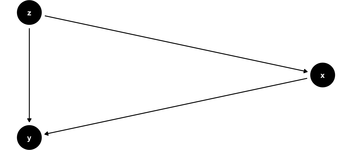
DAG example
In this figure, we have three variables, \(x\), \(y\) and \(z\). We can see that according to the plot, variable \(z\) causes variables \(x\) and \(y\), and variable \(x\) also causes variable \(y\). In the DAG jargon, we call the variables that cause other variables “parents” and the variables caused by others “children”. In our example, variable \(z\) is parent to variables \(x\) and \(y\). Variable \(y\) is a child of \(z\) and \(x\). Notice that the DAG doesn’t say anything about the nature of the relationships, it is merely a formal representation of their (presumed) existence.
Types of interferring variables
DAGs are useful for many things, one of which is that they allow us to develop a typology of interfering variables, which in turn allows us made an argument about which variables to control for in our analysis. Formally, we recognize four types of interfering variables:
- Counfounders
- Colliders
- Mediators
- Moderators
For example, consider we are interested in the relationship between knowledge about Covid and the probability a persons gets vaccinated. Does educating the public about Covid increases the number of people who get a vaccine shot and if so, by how much? Naively, we could just look the correlation between level of knowledge and the probability of vaccination.

Knowledge leads to behavior?
However, as the readers probably know, the reality is not that simple. The well-known phrase “correlation doesn’t imply causation” warns us that merely observing that people with more knowledge are more often vaccinated isn’t by itself enough to conclude that one leads to the other. For us to make this argument, we need to control for other variables of interest, to eliminate potential spurious relationships from our estimates. DAGs can help us choose which variables to control for.
Confounders
The first type of interfering variables are confounders, also known as the common parents or common causes. Consider our example of Covid knowledge and vaccination probability. On variable, that may also play a role in this relationship is socio-economic status of individuals in the study. Assume that higher socio-economic status leads to higher Covid knowledge, as people with higher status are better educated and more likely to watch news. Also assume that socio-economic status positively influences vaccination rate, perhaps because people with higher socio-economic status have more trust in public institutions and more need for travel, for which a vaccination is necessary. We could formaly visualize this in the following DAG.
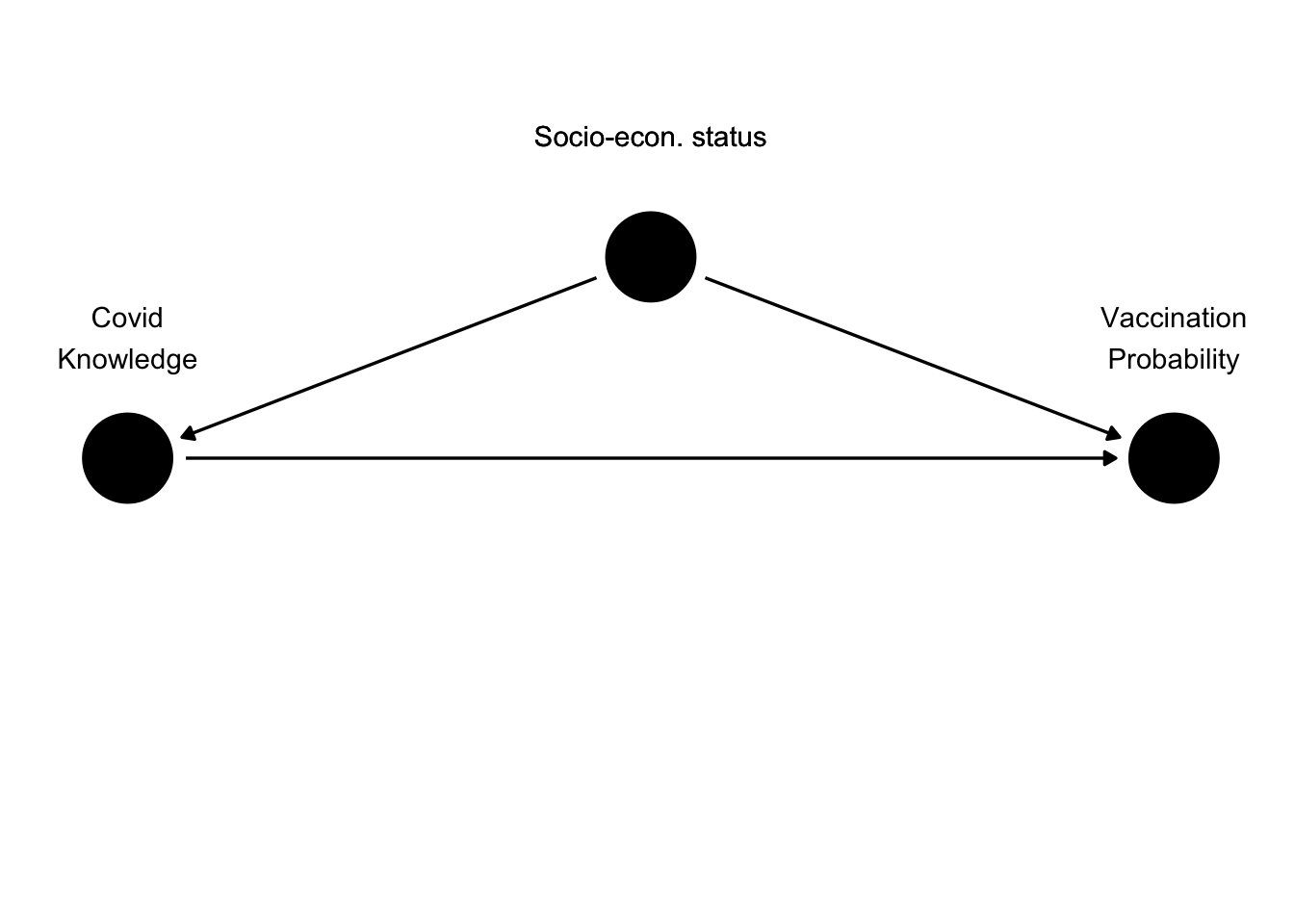
Socio-economic status as a confounder
What would this mean for our estimate of the relationship between knowledge and vaccination probability? If socio-economic status really raises both knowledge and vaccination rate, then there will be a positive correlation between both of them, as a raise in status will lead to a raise in both of its children. Consequently, if we want to get a good estimate of the true relationship between Covid knowledge and vaccination probability, we need to control for socio-economic status. In other words, we need to look at the relationship between the two variables only among people with the value of the confounder.
Readers will be probably familiar with other examples of confounding. One of the most popular is the relationship between the monthly number of drownings and the amount of ice cream sold, where the average temperature servers as a confounder. Generally speaking, we always want to control for all confounders, otherwise our results will be biased.
Colliders
Since not controlling for confounders leads to biased estimate of the relationship between our variables of interest, we may be tempted to control for as many variables as possible. Unfortunately, this isn’t a good strategy, as controlling for some variables may actualy make our model worse. These variables are called colliders.
Colliders are common children of two variables. Because the issue with colliders is not imminently obvious, we will look into a simple case first.
Imagine you are throwing two six sided dice. Both dice are fair and the throws are independent of each other. Knowing what is the value on the first die, can you the value of the second one?
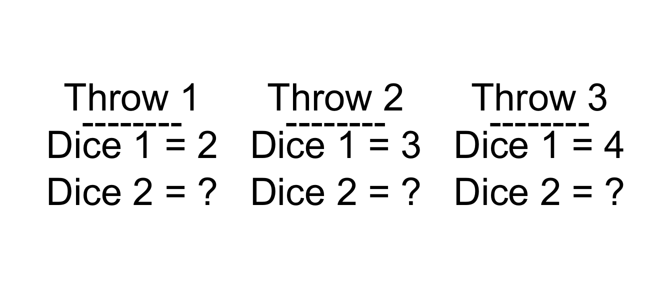
Throwing die
Since the two dice are independent, knowing the outcome of the first die doesn’t give us any information about the second. This translates in zero correlation between the values of the two dice, as expected.
Now let’s try this thought experiment again, but this time, we will know the sum of the values on both dice.
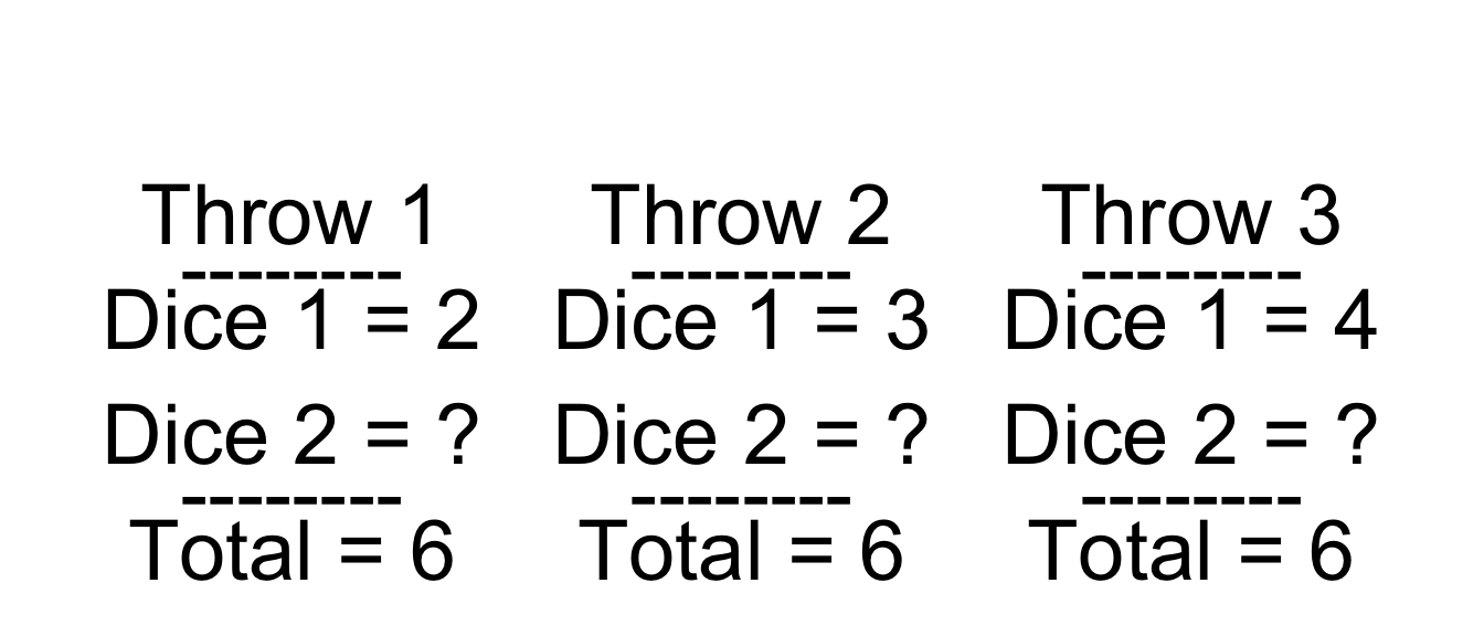
Throwing die again
Now we have more information. If the total number is 6, and the value on the first die is 2, then the number on the second die must be 4. Similarly, if the total is 6 and the value on the first die is 4, then the values on the second one must be 2. And so one. Quite logicaly, if the outcome of the throws is fixed, higher numbers on the first die must be compensated by lower numbers on the second. In other words, by controlling for the common outcome, we have created a negative correlation between two causally independent events.
Now we are ready to go back to our previous example. In the quest to estimate the effect of knowledge on vaccination probability, a researcher may want to control for whether an individual was previously hospitilized with Covid symptoms. This idea may be motivated by a desire to “filter out” the effect of hospitalization on vaccination acceptence or simply because controlling for hospitalization will greatly increase predictive power of the model. However, doing so would be inadvisable. First, let’s look at the DAG representation of the collider.

We may assume, as represented in the DAG, that hospitalization is the common outcome (common child) of both Covid knowledge and Vaccination probability. This is perhaps because being vaccinated makese the symptom of Covid less acute, which in turns lessens the need for hospitalization. At the same time, knowledge of Covid may also lower hospitalization rate, as more informed people are more likely to avoid situations where transmition is possible.
If these two assumptions are true, we encounter a variant of the dice problem. If a person belongs among the previously hospitalized and also among people with high Covid knowledge, the must almost surely haven’t been vaccinated. In the same vein, if a person belongs among previously hospitalized and also among people with high vaccination rate, they are almost surely among people with low Covid knowledge. Lastly, people with low knowledge and low vaccination probability are most likely to be hospitalized. The one combination we would almost never see is a person who was hospitalized, and yet has high Covid knowledge and high vaccination probability.
Looking only at the hospitalized people, i.e. controlling for hospitalization, could be potentionaly disasterous. In fact, it could be that by controlling for hospitalization, we would observe a strong negative correlation between knowledge and vaccination probability, even if the true causal relationship is strongly positive!
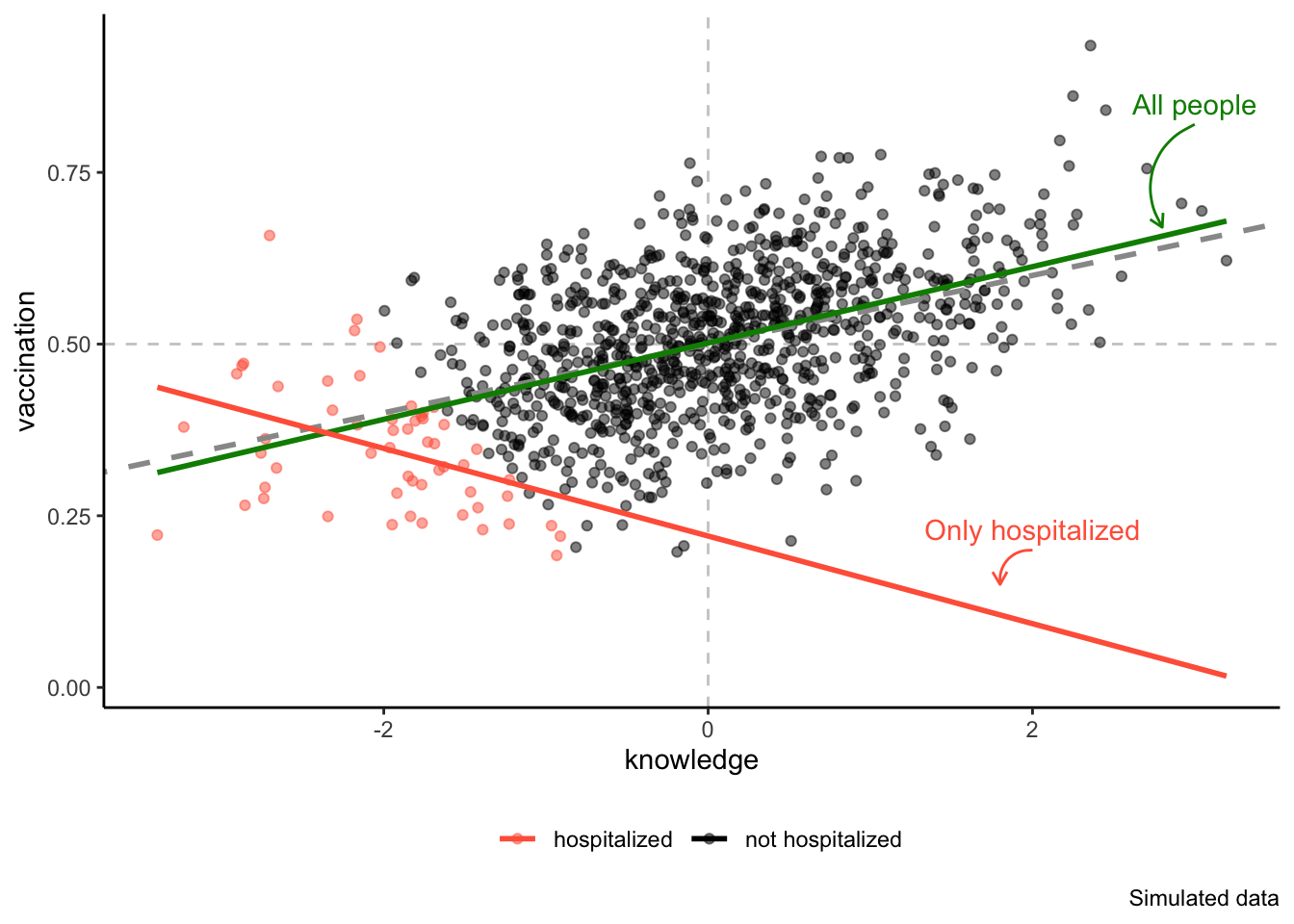
Don’t control for colliders
As the figure above shows, by controlling for hospitalization we would completely miss the true relationship between the two variables, represented by the dashed line. This illustrates that if our goal is explanative modeling, we must never control for colliders.
Mediators
Confounders and colliders are quite strict types of interfering variables, as their correct (not) inclusion is mandatory. Not including a confounder will always make our model worse, just as would including a collider. The next type of variables we are going to talk about, mediators, differs from them in the sense that adding them into our model may or may not be appropriate, depending on our research question.
Mediators are “intermediate steps” in the causal relationships between variables of interest. Causal effects are rarely direct, instead they often work through intermediates. A well known example would be the effect of gender on wages. While women have lower wages than men, it doesn’t mean that all men magically find more money in their accounts at the end of the month simply because they are men. Instead, the effect of gender is indirect. Gender may influence selection of the work industry, the probability of being a primary homemaker or behavior during job interviews. All these then determine persons wages.
In our Covid example, we may think about how exactly could knowledge of Covid influence the probability of vaccination. Perhaps increasing knowledge leads to perceive Covid as a bigger threat, essentially scaring them into getting vaccinated. This may be not the only causal pathway between knowledge and vaccination probability, but it may be a pathway of a special theoretical interest. We can represent mediators in our DAG as follows.
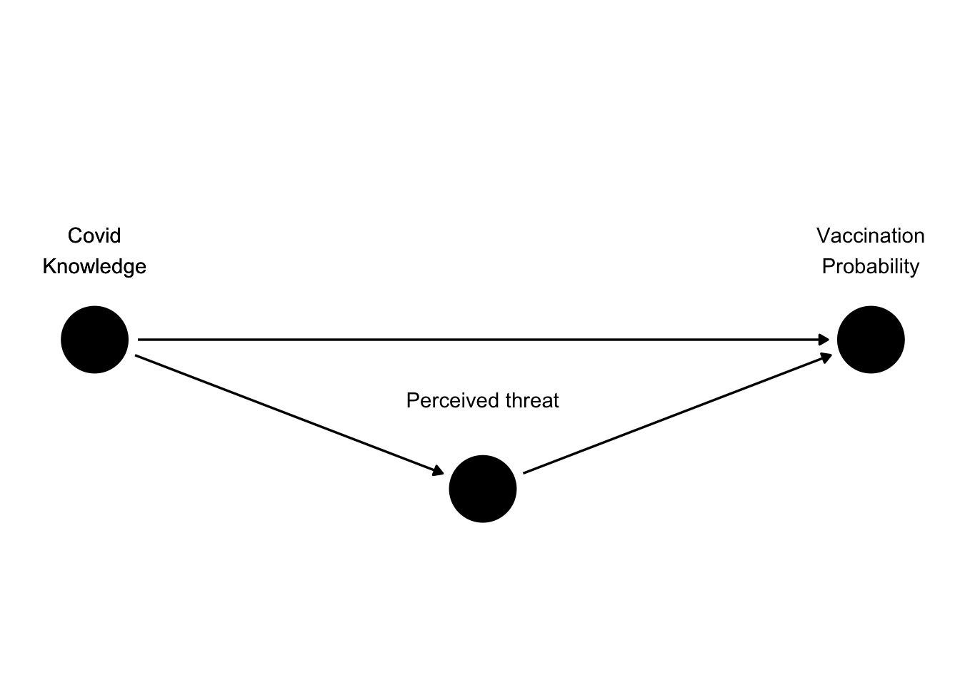
3
Notice that in the figure above, there are two paths through which knowledge influences vaccination probability. The first path is the direct one, straight from knowledge to vaccination. The other one is indirect, going through perceived threat of Covid. Whether we are interested in this indirect path depends on the goal of our analysis.
It is important to realize that by not adding perceived threat to our model, we are not necessarily making any error. Our estimate will simply be the total effect of knowledge on vaccination probability, including the effect of perceived threat as well as all other intermediate steps. If our research question was “What is the effect of knowledge on vaccination probability?” then adding mediators is simply not necessary. On the other hand, adding perceived threat allows to disentangle the effect of this specific intermediate step from all the others. This would be useful if our research question was “Does knowledge increase vaccination probability by raising perceived threat?” or “Are there other causal pathways between knowledge and vaccination probability other than perceived threat?”
In the context of linear regression, it’s important to remember that adding a mediator into our model changes the interpretation of regression coefficients. If the mediator is not present, we can interpret the regression coefficient as the total effect between variables. If the mediators is present, we interpret the coefficient as the direct effect, i.e. the effect not going through this specific indirect pathway. There are also more complex models, such as Structural equation models, that allows to examine indirect relationships in greater detail, but these are beyond the scope of this course.
Moderators
The last type of interfering variables are moderators. Moderators are not actualy part of the original DAG framework and their special in the sense that they don’t influence other variables, but the relationships between them.
Assume for example, that the accessibility of vaccination shots is not the same in all regions. In some regions, there may be fewer vaccination shots per person or fewer vaccination centers. In these regions, raising knowledge may not have much of an effect on vaccination probability, as the main limiting factor is supply. In other words, the effect of Covid knowledge on vaccination proability will be different depending on region. We can draw this fact into our DAG in the following way.
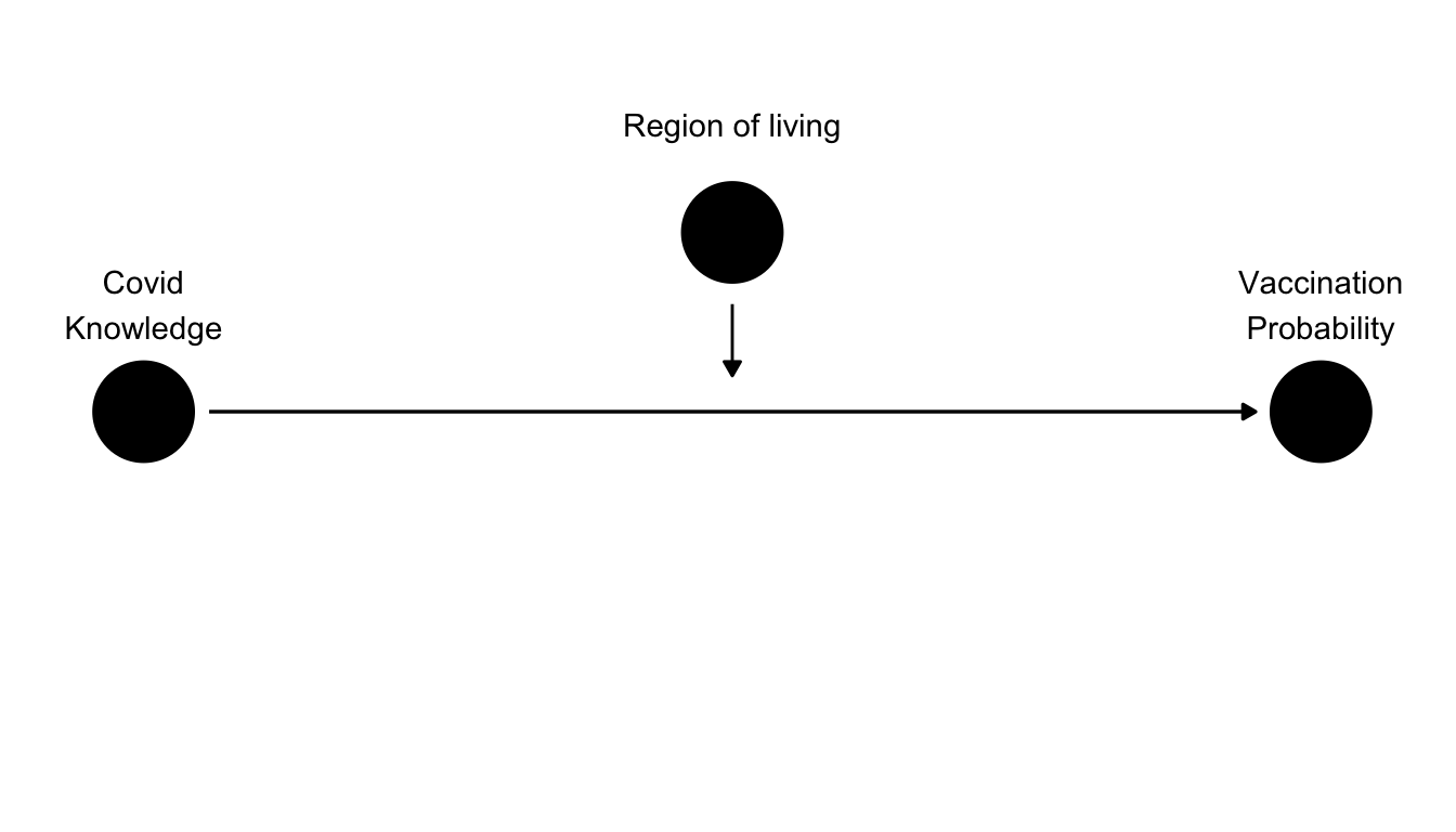
In context of linear regression, moderators are simply interactions between variables. Whether we want to consider adding an interaction to our model depends on our research question. If our goal is to estimate the average effect of knowledge on vaccination probability, no interaction is necessary. On the other hand, if we have a suspicion that there a great differences between regions and want to examine them, adding interaction (or moderator) between region and Covid knowledge would be appropriate.
Final DAG
By combining all the previous examples together, we will get the following DAG.
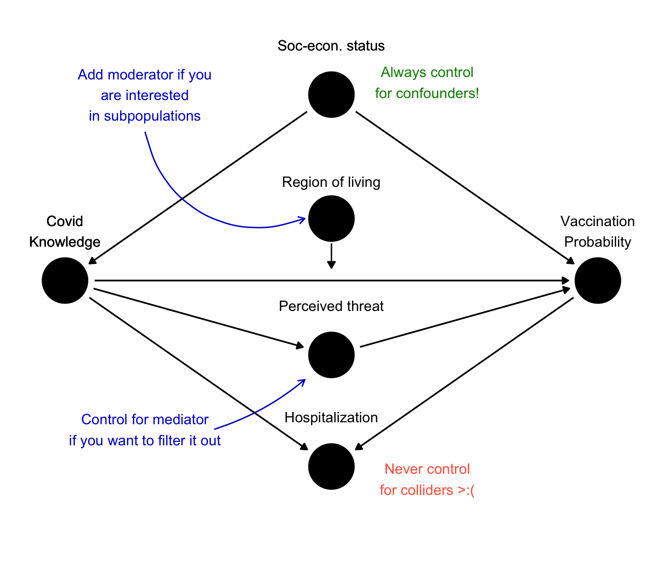
While maybe complicated at the first glance, DAGs like this can be a great help in deciding which variables to control for. We can identify confounder by the fact that they are common parents of our main variables of interest. Similarly, colliders will be common children. Mediators will lay somewhere between our two variables and moderators will point arrows to other arrows.
The main takeaway of this chapter is that you should always control for as many confounders as possible, while avoiding any colliders. Depending on your research question, you may want to add a mediator, to see if the direct effect persists even with it present. Lastly, if you are interested not only in the average effect, but also in sub populations, add moderator as an interaction.
Finaly, while drawing a DAG may be easily, drawing a good DAG may be very hard. Any specific DAG shouldn’t be based merely on how you guess the world works, but should be based on literature review and good knowledge of theory. DAGs are not a magic technique that would allow us to always draw causal inferences from observational data, but they are extremely useful due to the ability more clearly things about what exactly our models assume about the world.