Assumptions of linear regression
So far, we discussed how to create and interpret linear regression models. However, if we want to summarize complex relationships that exist in the real world using mathematical models, certain assumptions have to be made. The validity of our results then dependents on how well our models match these assumptions. In this context, it is important to note that no model can be at the same time both parsimonious and perfectly accurate, and therefore no assumption we can make regarding our models will ever be satisfied perfectly.
This does no mean that we should resign on the critical reflection of our models and blindly accept whatever results they may give. On the contrary, we should think carefully about the ways in which our models deviate from the assumptions we established and what consequences these deviations may have. As the british statistician George E. P. Box (allegedly) said: “All models are wrong, but some are useful”.
The most important assumptions of linear regression model, in order of relative importance, are as follows (Gelman et al., 2020).
1. Validity
The most important, and at the same time most elusive, is the assumption of validity, which relates both to the variables of interest and the model itself. Firstly, we should make sure that the data we use are sufficient to answer the research question at hand. This often becomes a problem in secondary analyses, in which we reuse data from previous studies. Since no two studies have the same goal, data gathered by other researchers will probably not align perfectly with our research questions, and consequently important variables may be missing or not be measured in sufficient detail.
Secondly, all traits and phenomena we want to analyze need to be measured with sufficient quality. Theoretical constructs have to be operationalized adequately, so that we don’t miss any of its important facets and, if possible, validated measuring tools should be used, to make sure that our measurement is both reliable and valid. We should also be careful not to mistake related traits with each other. For example, it may be tempting to use school grades as a measure of academic proficiency, but grades are often influenced not by academic skills, but also by behavior and personal traits of students and hence may not be an ideal proxy.
Thirdly, data must be gathered in such way that inference to the desired population is possible. A sample of university students may be fine if our goal is to learn about this specific population, but we should be careful about generalizing to any more general group. In the similar vein, a representative sample of Czech population may not be ideal if our goal is to study a narrowly specified subset, such as second generation immigrants.
Lastly, our models has to be correctly specified to capture the true relationships between variables. If we were to specify a linear relationship between age and income, when in reality the two variables would be nonlinear dependent, our conclusions would be biased. To correctly specify a model, we can either lean on theory to guide us or make our model sufficiently flexible so that we don’t introduce unreasonable assumptions about the nature of the studied topic.
Overall, while it is impossible to design a perfect study, which would fully satisfy all facets of validity, we should strive to do as well as possible, as the loss of validity strongly lessens the usefulness of our findings.
2. Representativeness
The second assumption is the one of representativeness If our goal is either prediction or inference, our data needs to be a representative sample of the population of interest. More specifically, we assume that the distribution of the dependent variable is representative of the population, given the the predictors. This is a distinction with an important implication. While it is crucial for the dependent variable to be sampled in representative manner, it is not strictly necessary for the the rest of the variables in the model. Consider for example model predicting income based on age:
\[ income = \beta_0 + \beta_1*age+\epsilon \]
Ideally, we would have sample representative in both age and income, as shown in the subplot A below. Notice however, that even if we only sampled respondents with above average age, the estimated relationship between age and income would still be identical to the one from the fully representative sample (subplot B). Only in the situation where the sampling is biased in term of income, would our inference be significantly of (subplot C). The red line shows the true relationship between the variables, while the blue one shows the relationship on the reduced data set.
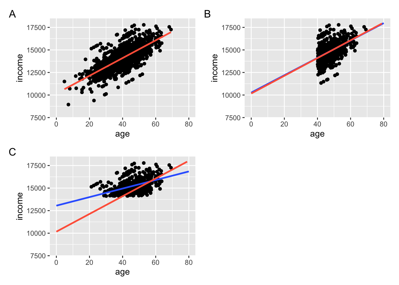
Example of A) Fully representative sample, B) Sample with indepdendent variable bias c) Sample with dependent variable bias
This also naturally extends to undersampling and oversampling. Oversampling older respondents would be of little worry, while oversampling respondents with low income would be a considerable problem. We should therefore pay special attention to potential sampling biases regarding our dependent variables, especially if our goal is inference.
3. Linearity and additivity
The first and the most important mathematical assumption of linear regression are the assumptions linearity and additivity. All linear models assume that the expected value of the dependent variable can be computed as a linear combination of predictor values and their regression coefficients:
\[ y = \beta_0 + \beta_1*x_1 + \beta_2*x_2\:+\:...\:\beta_p*x_p \]
Not all relationships are necessarily additive and linear An example of a multiplicative model would be:
\[ y = \beta_0 + (\beta_1*x_1) * (\beta_2*x_2) \]
As a rule of thumb, if the regression coefficients in the model are only either add or subtracted from each other (i.e. \(\beta_1*x_1+\beta_2*x_2+...)\)), the model is considered linear and additive. On the other hand, if the regression coefficients are multiplied, divided or taken to the power of each other, the relationship the model is either not linear or not additive.
Just because some relationships are not linear in their natural form, all is not lost. Perhaps confusingly, some nonlinear models can be transformed into a linear form, using an appropriate transformation. One of the widely used transformation are logarithms, which can ,roughly speaking, convert multiplication to addition and division to subtraction. Consider the example of the multiplicative model above. We can transform such model into linear form by simply taking the logarithm of the product, as the logarithm of product is the sum of logarithms:
\[ \beta_0 + log[(\beta_1*x_1) * (\beta_2*x_2)] = \beta_0 + log(\beta_1*x_1) + log(\beta_2*x_2) \]
The assumptions of linearity and additivity are crucial, as linear models can only capture relationship which fulfill these assumptions. While no relationship between two variables is perfectly linear in the real world, many can be approximated in such way. Despite this, we should be careful about parametrizing our models, as failing to at least approximately fulfill these assumptions biases both our regression coefficients and our predictions, and thus presents danger no matter what our goals are. For examples on how can a volition of these assumptions lead to incorrect conclusions, see (King & Roberts, 2015).
4. Independence of errors
Another important assumptions is that the errors, i.e. the differences between the true and the predicted values, are independent of each other. This assumption is often violated in time series, where the errors at the time of t are correlated with the errors at the time of t-1 (or t-2, t-3, etc.). In other words, values that are measured closer together in time have more similar values of errors. Such thing can also happen in analysis of spatial data, where regions that are geographically close together have similar errors. The violation of this assumption leads to incorrect estimation of standard error, and therefore presents a risk to inference (Williams et al., 2019).
5. Homoscedasticity (constant variance of errors)
The standard linear regression is derived under the assumption that the errors have the same variance across all levels of the dependent variable and such situation is called homoscedasticity. If the variance of the errors is not constant, the the error are heteroscedastic.
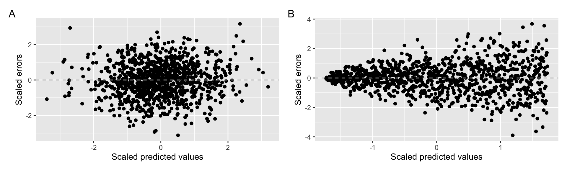
Example of A) homoscedastic data B) heteroscedastic data
The violation of this assumption has two consequences (White, 1980). Firstly, the estimation of the regression coefficients become inefficient. This simply mean that we will need bigger sample size to obtain the level of precision than if the the errors were homoscedastic. The second, more serious problem is that the estimates of the standard errors of the coefficients would be biased, leading to incorrectly specified p values and standard errors. Therefore, this assumption is most important when our goal is inference or in situations where the precision of estimates matters greatly (e.g. when we are estimating weak relationships or small effect sizes).
6. Normality of errors
The last of the assumptions states that the errors should be normally distributed. This is especially important for the prediction of individual observations, i.e. if our goal is to predict values of individual persons rather than just the average value. Furthermore, the normality of residuals is important for the inference from small samples. The classic way of inference assume that the sampling distribution of regression coefficients is normal. This assumption can be assured in several way, one of which is that the errors itself have normal attribution. On the other hand, for large enough samples, the sampling distribution of regression coefficient will approach normality no matter the distribution of residuals (Lumley et al., 2002; Schmidt & Finan, 2018). Therefore, the assumption of normality is only needed when the prediction on the individual level is desired or when we seek inference from small samples.