Multiple linear regression
The goals for this lecture are (1) understanding the concept of multiple linear regression with emphasis on interpretation of its coefficients, and (2) building and interpreting multiple regression models in R.
Introduction to multiple linear regression
Multiple linear regression (MLR) is defined as having multiple predictor terms (more than one). Remember the general formula for simple linear regression:
\[ Y = \alpha + \beta*X + \epsilon, \] where \(\alpha + \beta*X\) represents the line and \(\epsilon\) represent the deviation from it.
The formula for MLR is its fairly straightforward extension. Notice that intercept in MLR is usually called \(\beta_0\) rather than \(\alpha\). The other regression coefficients are numbered betas. The numbered x-es stand for predictor terms.
\[ Y = \beta_0 + \beta_1*x_1 + + \beta_2*x_2 + ... + \epsilon \]
Appreciate that having more predictor terms does not necessarily imply using more predictor variables. For example, the blue line in the following figure represents linear model estimated using three predictor terms: democratic index, democratic index to the power of two (quadratic term), and democratic index to the power of three (cubic term). While the model only uses one predictor variable, there are three predictor terms which makes the model a case of MLR (the interpretation framework of MLR explained in this lecture applies). For this model, four betas would be estimated (one of them the intercept).

One of the common misconceptions about linear regression is that it can only estimate a straight line. That is only true for simple linear regression. From the picture above, it should be clear that in MLR, it is possible to “bend” the line. And not only that. Throughout the course we will see how flexible MLR can be.
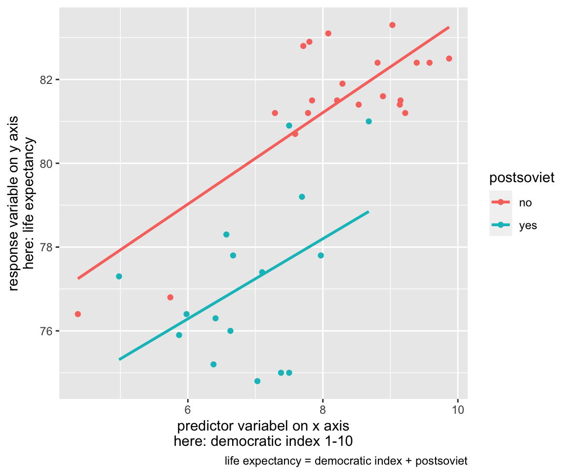
Another example of a MLR model is visualized on the figure below. It uses two predictor terms (in this case, they are two distinct independent variables): again, the democratic index, and, in addition, a binary variable whether the country is post-soviet or not. Due to the fact that one of the independent variables is binary, it is possible to visualize the whole model in one two-dimensional figure as two lines. However, more complex MLR models cannot be meaningfully visualized on top of the raw data.
Interpreting coefficients in MLR
First, let’s run a model where life expectancy is explained with democratic index and percentage of people with university degree in 15-64 age category (that is how the variable is defined so we just use what we have).
fit1 <- lm(life_exp ~ dem_index + uni_prc, data = countries)
summary (fit1)
##
## Call:
## lm(formula = life_exp ~ dem_index + uni_prc, data = countries)
##
## Residuals:
## Min 1Q Median 3Q Max
## -4.1640 -0.9798 -0.0910 1.4256 3.1522
##
## Coefficients:
## Estimate Std. Error t value Pr(>|t|)
## (Intercept) 66.300 2.210 30.003 < 2e-16 ***
## dem_index 1.786 0.415 4.303 0.000149 ***
## uni_prc -1.460 6.548 -0.223 0.824979
## ---
## Signif. codes: 0 '***' 0.001 '**' 0.01 '*' 0.05 '.' 0.1 ' ' 1
##
## Residual standard error: 1.949 on 32 degrees of freedom
## (3 observations deleted due to missingness)
## Multiple R-squared: 0.5517, Adjusted R-squared: 0.5237
## F-statistic: 19.69 on 2 and 32 DF, p-value: 2.664e-06The output above should look familiar, it differs from that of simple linear regression (previous lecture) only by having an extra row in the coefficient table. The beta coefficients are in the column called “Estimate”. Specifically, the coefficient for democratic index is 1.786 (recall that the coefficinet was 1.62 when democratic index was the only predictor), and the coefficient for university education is -1.460.
Interpreting coefficients in MLR can be surprisingly tricky as they are, “in part, contingent on the other variables in the model” (Gelman et al., 2020, p. 131). This means that they will change when other variables are added to the model or dropped from the model.
We will cite Gelman et al. (2020) on how best to interpret them: “The coefficient \(\beta_k\) is the average or expected difference in outcome \(y_k\), comparing two people who differ by one unit in the predictor \(x_k\) while being equal in all the other predictors. This is sometimes stated in shorthand as comparing two people (or, more generally, two observational units) that differ in \(x_k\) with all the other predictors held constant” (p. 131). We also call this conditional effect (as in “conditional on the assumption that all other predictors are held constant”).
For the example above, we could say that if one country has democratic index higher by one point than another country, and they both have the same percentage of university educated people, the first country will have expected life expectancy higher by 1.8 years (we encourage to reasonably round the beta of 1.786 for interpretation purposes to avoid making impression of unjustified precision).
Since the coefficient for percentage of university educated people
has very broad confidence interval (and very high p-value), we could
also say that we find no evidence in the data, that two countries with
the same level of democratic index should be expected to differ in life
expectancy when they have different proportion of university educated
people. That is if we believe the sample of countries justifies some
generalization to some concrete or at least abstract population of
countries. Someone could be tempted to make a purely descriptive
interpretation with no ambition to make sample-to-population inference.
He or she could try to say something along the lines that for our
particular sample of countries and data from given years, we find that
for two countries with the same level democratic index the life
expectancy goes down by 1.46 years, on average, as the proportion of
university educated increases from 0 to 100% (the variable is measured
on scale from 0 to 1). This seems to us a meaningless statement and we
would discourage from it, even if technically true. The really large
standard errors should warn us against making interpretation even in
purely descriptive situations. Saying that controlling for democratic
index, there does not seem to be any linear association between life
expectancy and proportion of university educated in our sample of
countries seems much more sensible.
Within descriptive modeling strategies, we use MLR to see the effects of individual variables net of the effects of all the other predictors in the model. Within predictive modeling, we use MLR to improve our predictions over simple linear model (predictions based on just one predictor term often tend to be weak in social sciences). Within explanatory modeling, we use MLR for adjusting for background variables according to our theory, hence discovering potentially spurious relationships and isolating potentially causal effects.
Difference-based vs. change-based interpretations
There are two conceptually slightly different interpretations of MLR coefficients. The difference-based interpretation is well described as “how the outcome variable differs, on average, when comparing two groups of items that differ by 1 in the relevant predictor while being identical in all the other predictors” (Gelman et al., 2020, p. 134). In contrast, the change-based interpretation is well described by saying that “the coefficient is the expected change in y caused by adding 1 to the relevant predictor, while leaving all the other predictors in the model unchanged” (Gelman et al., 2020, p. 134).
In others words, the difference-based interpretation uses the idea of difference between individuals, whereas the change-based interpretation uses the idea of change within individual. To be on the save side, we recommend interpreting regression coefficients as comparisons between units, not (potential) changes within units, unless one specifically claims causality. The difference-based interpretation is simply more general, hence carries less risk of being used in a misleading way. (By misleading we mean invoking causality where no evidence for a causal relationship is shown.)
Note that (Gelman et al., 2020) use the term “predictive interpretation” instead of difference-based interpretation and “counterfactual” interpretation instead of change-based interpretation.
Comparing beta coefficients of different predictors
It can be sometimes useful to compare coefficients of different independent variables in the model. As we saw in the model above, it cannot be done in a straightforward way. While values of 1.786 and 1.460 are not very far from each other, it makes no sense to compare them. The first shows change when two countries differ in democratic index (measured on the scale from 0 to 10) by one (a realistic situation), whereas the latter shows change when one country has no university educated people and the other has only university educated people (a very unrealistic situation). Indeed, the coefficient value depends on the unit we use for measuring the independent variable.
To deal with this issues of no comparability, we can use so called standardized betas. Those can be used to determine relative weight or strength of independent variables as they show the effect of an increase in X by one standard deviation on Y, also measured in standard deviations. The way to calculate standardized betas is to first standardize (compute z-scores) all variables used in the model and then run a regression on the z-scores.
A way to do this using the scale function directly in the regression call is shown below.
fit2 <- lm(scale(life_exp) ~ scale(dem_index) + scale(uni_prc), data = countries)
summary (fit2)
##
## Call:
## lm(formula = scale(life_exp) ~ scale(dem_index) + scale(uni_prc),
## data = countries)
##
## Residuals:
## Min 1Q Median 3Q Max
## -1.47433 -0.34693 -0.03223 0.50475 1.11609
##
## Coefficients:
## Estimate Std. Error t value Pr(>|t|)
## (Intercept) -0.02280 0.11802 -0.193 0.848054
## scale(dem_index) 0.82340 0.19138 4.303 0.000149 ***
## scale(uni_prc) -0.04001 0.17945 -0.223 0.824979
## ---
## Signif. codes: 0 '***' 0.001 '**' 0.01 '*' 0.05 '.' 0.1 ' ' 1
##
## Residual standard error: 0.6899 on 32 degrees of freedom
## (3 observations deleted due to missingness)
## Multiple R-squared: 0.5517, Adjusted R-squared: 0.5237
## F-statistic: 19.69 on 2 and 32 DF, p-value: 2.664e-06Now we can compare the relative strengths of our predictors. The democratic index (with standardized beta of 0.82) is a way stronger predictor of life expectancy than the proportion of university educated (0.04 in absolute value as the sign is irrelevant for this comparison). Notice that the values of t-tests for the significance of coefficients did not change. It should come as no surprise, we did not substantively change the data by standardizing it. Also remember that we are comparing the net effect of the predictors. The comparison could look quite different when standardized betas from two simple linear regression models were compared.
Gelman (2008) suggests to use slightly different transformation if we also want include binary predictors (dummy variables) in the model. He shows that standardizing by subtracting the mean and dividing by 2 standard deviations (rather than just 1) enables to directly compare this kind of standardized betas with coefficients for non-standardized binaries.